Flattening Not Fattening The Curve

Flattening not Fattening the Curve

[2020-03-23]

COVID-19 caused by SARS-CoV-2 is a global pandemic. It is causing deaths skewed towards the older demographic, and damaging economies worldwide.

The biggest threat and reality of this disease is the over saturation of medical facilities beyond their carrying capacities resulting into sub-optimal patient care and ultimately high death rates.

The intrinsic capacity of SARS-CoV-2 to enter the human body is hard to control but the rate at which it can spread through populations (transmission rate) is much more feasible for us to manipulate.

The key is time. That is reduce the infection rate and the spread of the disease and therefore inhibit the over saturation of medical facilities and save lives.

Let’s say for example we get an instantaneous (one time right now) measurement of the rate of infection = dN/dt, that is how many people are being infected per unit time. Now being in the real-world, we know that this rate should be regulated by total number of people that can be infected. Hence we model this instantaneous infection rate simplistically as:

dN_over_dt = function(rate, N, K){
  rate*N * (1-(N/K))
}

where:

• rate is the transmission rate or the number of people a person can infect
• N is the number of infected people
• K is the maximum number of people that can be infected - our limiting factor. We can see that from this differential equation the rate of infection approaches zero as N approaches K. Now solving this differential equation to get the cumulative number of infections or cases we get the familiar logistic function:

  N_t = function(time, rate, N_0, K){
    C_0 = (K - N_0) / N_0
    N_t = K / (1 + C_0*exp(-rate*time))
    return(N_t)
  }
  

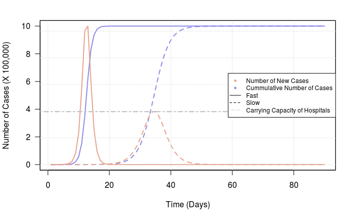
  Assuming the total number of people that can be infected is capped at one million (fingers-crossed or lower obviously):

  K = 1e6
  

  Also let’s say that we start with a single person being infected:

  N_0 = 1
  

  And that we have control measures that reduce or exacerbates transmission rates:

  rate_slow = 0.4
  rate_fast = 1.1
  

  Predicting the cumulative number of cases and the rate of new cases for 3 months since the initial infection we get:

  time = seq(from=1, to=90, by=1)
  n_cases_slow = N_t(time, rate_slow, N_0, K)
  n_cases_fast = N_t(time, rate_fast, N_0, K)
  plot(x=c(min(time), max(time)), y=c(min(c(n_cases_slow, n_cases_fast)), max(c(n_cases_slow, n_cases_fast)))/1e5, type="n", xlab="Time (Days)", ylab="Number of Cases (X 100,000)", las=1)
  lines(x=time, y=n_cases_slow/1e5, lty=2, lwd=2, col=rgb(0.5,0.5,0.9,alpha=0.9))
  lines(x=time, y=n_cases_fast/1e5, lty=1, lwd=2, col=rgb(0.5,0.5,0.9,alpha=0.9))
  par(new=TRUE)
  rate_cases_slow = dN_over_dt(rate_slow, n_cases_slow, K)
  rate_cases_fast = dN_over_dt(rate_fast, n_cases_fast, K)
  plot(x=c(min(time), max(time)), y=c(min(c(rate_cases_slow, rate_cases_fast)), max(c(rate_cases_slow, rate_cases_fast))), type="n", xaxt="n", yaxt="n", xlab="", ylab="")
  lines(x=time, y=rate_cases_slow, lty=2, lwd=2, col=rgb(0.9,0.6,0.5,alpha=0.9))
  lines(x=time, y=rate_cases_fast, lty=1, lwd=2, col=rgb(0.9,0.6,0.5,alpha=0.9))
  grid()
  abline(h=max(rate_cases_slow), lty=4, lwd=2, col="gray")
  legend("right", 
      legend=c("Number of New Cases", "Cummulative Number of Cases", "Fast", "Slow", "Carrying Capacity of Hospitals"),
      pch=c(20,20,NA,NA,NA),
      lty=c(NA, NA, 1, 2, 4),
      col=c(rgb(0.9,0.6,0.5,alpha=0.9), rgb(0.5,0.5,0.9,alpha=0.9), "black", "black", "gray"),
      cex=0.75
      )