Climate Data From Bom

Climate data from the Bureau of Meteorology (BOM) of the Australian government

Publicly available climate information is available from the Bureau of Meteorology.

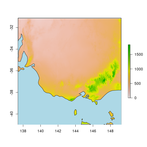
We can visiualise and extract this information in R like so using mean annual rainfall in southeast Australia:

> print(cropped@data@values)
[1] 1414.06

The Rscript used to accomplish this is:

library(maps)
library(raster)

### Load the rainfall data, in grid format which can have a *.txt or *.asc extension name
rainfall = raster::raster("bom_grid_data_1991_to_2020/rainan.asc")

### Crop the area of interest
x_limit = c(137.4154, 149.2455)
y_limit = c(-40.90563, -31.15542)
e = as(raster::extent(x_limit[1], x_limit[2], y_limit[1], y_limit[2]), 'SpatialPolygons')
raster::crs(e) = "+proj=longlat +datum=WGS84 +no_defs"
rainfall = raster::crop(rainfall, e)

### Plot
plot(rainfall)
outline = maps::map("world", plot=FALSE)
xrange = range(outline$x, na.rm=TRUE)
yrange = range(outline$y, na.rm=TRUE)
xbox = xrange + c(-2, 2)
ybox = yrange + c(-2, 2)
### draw the outline of the map and color the water blue
polypath(c(outline$x, NA, c(xbox, rev(xbox))),
        c(outline$y, NA, rep(ybox, each=2)),
        col="light blue", rule="evenodd")
grid()

### Extract a data point for a specific location
x = 146.4754 ### longitude coordinate of the location of interest
y = -36.17938 ### latitude coordinate of the location of interest
epsilon = 1e-8 ### a cute number to define tiny area
e = as(extent(x-epsilon, x+epsilon, y-epsilon, y+epsilon), 'SpatialPolygons')
crs(e) = "+proj=longlat +datum=WGS84 +no_defs"
cropped = crop(data_env, e)
print(cropped@data@values)