Autoregression Vs Smooth Splines For Spatial Analysis

Autoregressive models vs smoothing splines for spatial analysis

[2024-10-17]

Let’s take a look at the differences between using autoregression and smooth spline to fit spatial effects in a mixed linear model context.

### Load the spatial data
library(sommer)
data(DT_yatesoats)
df = DT_yatesoats
df$row_factor = df$row
df$col_factor = df$col
df$row = as.numeric(df$row)
df$col = as.numeric(df$col)
str(df)
### Autoregressive model
model_ar = sommer::mmer(
  fixed = Y ~ 1 + V,
  random = ~ row_factor + col_factor + sommer::AR1(row_factor:col_factor),
  rcov = ~ units,
  data = df,
  dateWarning = FALSE,
  verbose = TRUE
)
### Smooth spline model
n_rows = length(unique(df$row))
n_cols = length(unique(df$col))
model_sp = sommer::mmer(
  fixed = Y ~ 1 + V,
  random = ~ row_factor + col_factor + sommer::spl2Da(x.coord=row, y.coord=col, nsegments=c(n_rows, n_cols), degree=c(3,3)),
  rcov = ~ units,
  data = df,
  dateWarning = FALSE,
  verbose = TRUE
)
### Did the models converge? Yes.
model_ar$convergence
model_sp$convergence
### How well-fit are the models? The smoothing spline model is slightly better than the autoregressive model, i.e. higher likelihood and lower AIC and BIC
summary(model_ar)$logo
summary(model_sp)$logo
summary(model_ar)$logo$logLik > summary(model_sp)$logo$logLik
summary(model_ar)$logo$AIC < summary(model_sp)$logo$AIC
summary(model_ar)$logo$BIC < summary(model_sp)$logo$BIC
### Are the variance components non-zero? Yes.
summary(model_ar)$varcomp
summary(model_sp)$varcomp
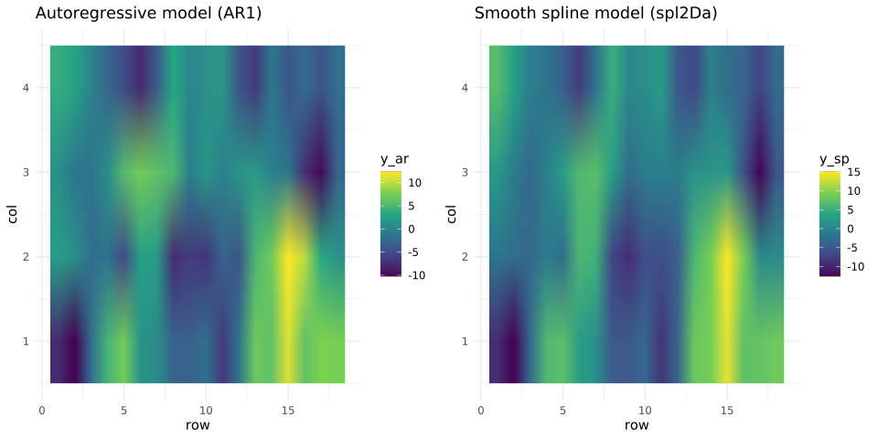
### What are the fitted values? See below including the heatmaps.
df_fitted_ar = fitted.mmer(model_ar)$dataWithFitted
df_fitted_ar$y = df_fitted_ar$`sommer::AR1(row_factor:col_factor).fitted`
str(df_fitted_ar)
df_fitted_sp = fitted.mmer(model_sp)$dataWithFitted
df_fitted_sp$y = df_fitted_sp$`A:all.fitted`
str(df_fitted_sp)
### Merge the fitted values for the interaction of spatial terms
df_fitted_merged = merge(
    data.frame(row=df_fitted_ar$row, col=df_fitted_ar$col, y_ar=df_fitted_ar$y),
    data.frame(row=df_fitted_sp$row, col=df_fitted_sp$col, y_sp=df_fitted_sp$y),
    by=c("row", "col")
)
### Distribution differences? Yes, there is more variation in the smooth spline model.
var(df_fitted_merged$y_ar)
var(df_fitted_merged$y_sp)
txtplot::txtdensity(df_fitted_merged$y_ar)
txtplot::txtdensity(df_fitted_merged$y_sp)
### Plot
library(ggplot2)
p_ar = ggplot2::ggplot(data=df_fitted_merged, aes(x=row, y=col, fill=y_ar))
p_ar = p_ar + geom_raster()
p_ar = p_ar + scale_fill_viridis_c()
p_ar = p_ar + theme_minimal()
p_ar = p_ar + labs(title="Autoregressive model (AR1)")
p_sp = ggplot2::ggplot(data=df_fitted_merged, aes(x=row, y=col, fill=y_sp))
p_sp = p_sp + geom_raster()
p_sp = p_sp + scale_fill_viridis_c()
p_sp = p_sp + theme_minimal()
p_sp = p_sp + labs(title="Smooth spline model (spl2Da)")
svg("sommer_spatial_AR1_vs_spl2Da.svg", width=10, height=5)
gridExtra::grid.arrange(p_ar, p_sp, nrow = 1)
dev.off()

From this example, we can say that smooth spline has slightly better fit than the autoregressive model. The smooth spline yields higher variance in the random effects but the resulting fitted values are smoother than the autoregressive model. An alternative way to interpret this is that with smooth spline models, there is lower probability of identifying artifacts, i.e. small intense peaks and troughs.